Diffusion models

The forward pass (image to noise)

The forward process can be described with a sequence of gaussian distributions:

Assume $\beta_t$ is the weight for gaussian noise (variance) at step $t$, and $\alpha_t = 1 - \beta_t,~ \bar\alpha_t= \prod_{i=1}^t\alpha_i$.

The forward step gradually adds a sequence of gaussian noise $\{\epsilon_t\} \sim \mathcal N(0, I)$ to the real image $x_0$, so the corrupted image at step $t$ is:

Note that two independent gaussian noise $\epsilon_{1}, \epsilon_{2}$ can be merged into one:

This means we can express any $x_t$ with $x_0$, $\{\beta_1, \beta_2, \cdots, \beta_t\}$, and a random noise $\epsilon_{t}$.

The backward pass (noise to image)

Given $x_{t}$, we want to get $x_{t-1}$, and eventually restore the real image $x_0$.

It's proven that if $\beta_t$ is small enough, the backward process is also a sequence of gaussian.

which gives the denoising step with another sequence of gaussian noise $\{z_t\} \sim \mathcal N(0, I)$:

Through some math we could get:

Note that here $\epsilon_t$ is the exact noise added in the forward step!

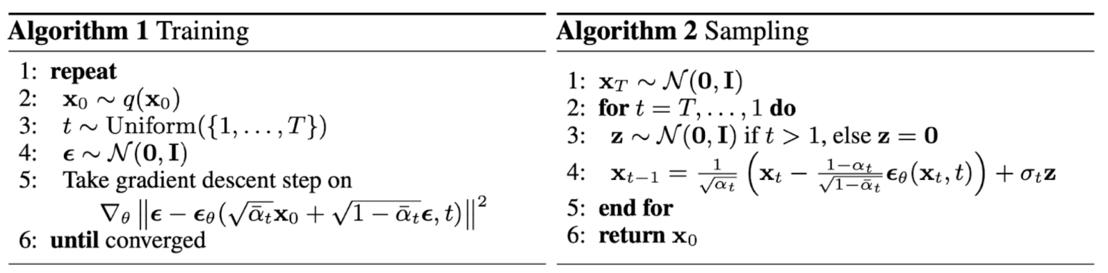
And all we need is a neural network that predicts this noise $\epsilon_t$ given $x_t(x_0, t) = \sqrt{\bar \alpha_{t}}x_{0}+\sqrt{1-\bar \alpha_{t}}\epsilon_t$.

Assume the predicted noise is $\epsilon_\theta$, we need to minimize the following loss:

The neural network is usually an U-Net with attention since we need same-size output as input.

DDPM (Denoising Diffusion Probabilistic Model)

DDPM exactly describes the above idea.

Note that DDPM use $\tilde \beta_t = \beta_t$ as an approximation.

DDIM (Denoising Diffusion Implicit Model)

DDIM use a different formula for the backward step:

According to $x_{t-1} = \tilde\mu_t(x_t, t)+\tilde \beta_t z_t$, we have

Another hyper-parameter $\eta \ge 0$ is introduced as $\eta \tilde \beta_t = \sigma_t^2$.

DDPM usually requires $T=1000$ steps for both training and inference ($S = T = 1000$), which makes generation (inference) too slow.

To speed up inference, DDIM use strided sampling where $S <T$, and shows when $\eta = 0$, $S=50\sim100$ steps are enough to generate good images.

LDM (Latent Diffusion Model)

Instead of diffusing in the pixel space, LDM first use a VQVAE to compress the image space (e.g., 512x512x3) into a latent space (e.g., 64x64x4).

This greatly reduces the computation cost for both training and testing.

Conditioned Generation

Assume we want to condition the generation to an input $y$ which may be class labels or text.

Classifier-Guided Diffusion

A pretrained classifier is required, not flexible.

Classifier-Free Guidance

Train both conditioned denoiser $\epsilon_\theta(x_0, t)$ and unconditioned denoiser $\epsilon_\theta(x_0, t, y)$ in the same neural network together.

The final denoiser is simply a weighted combination of these two terms:

where a larger $w$ leads to stronger class guidance.